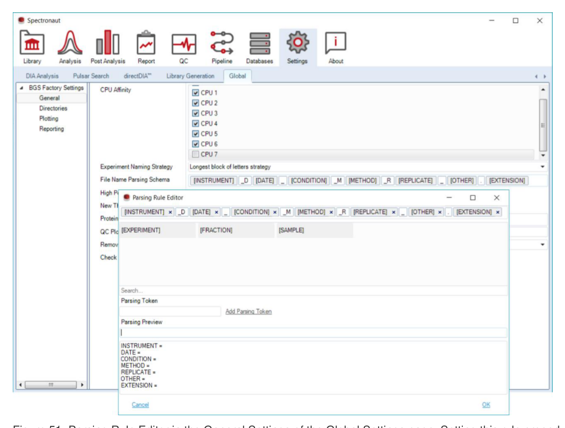
重点:用于固定本地路径、CPU 使用范围和稳定运行环境。
Spectronaut 图谱
本页收录 Figure 1-108 全部界面图、图谱与示意图,按模块分组,用于操作定位、结果判读、字段回查和附录复核。
图组
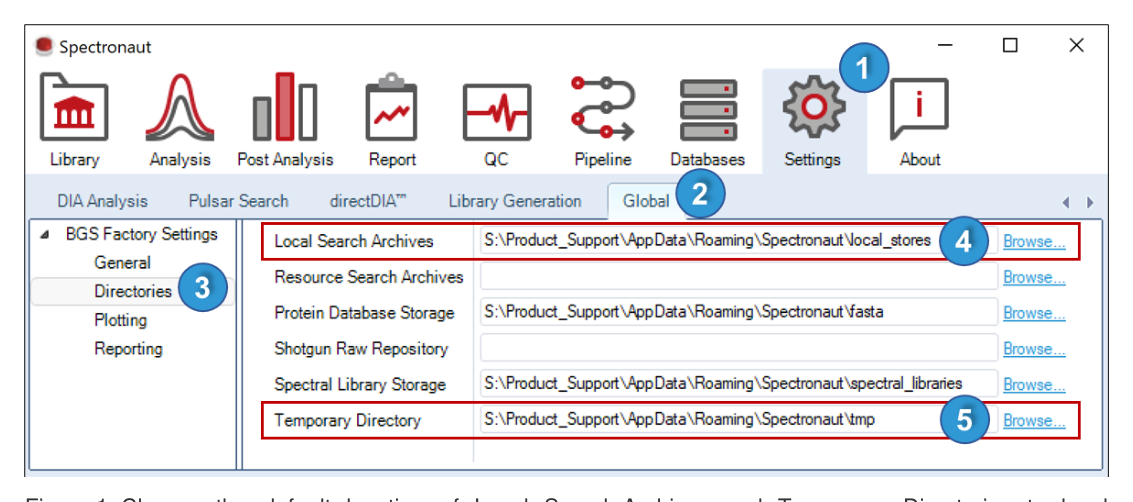
软件定位、目录规划、CPU 与本地资源设置。
重点:用于固定本地路径、CPU 使用范围和稳定运行环境。
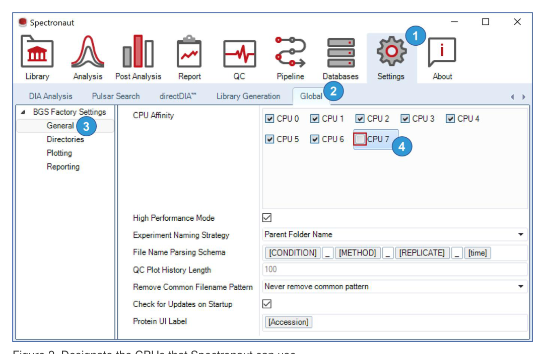
重点:用于固定本地路径、CPU 使用范围和稳定运行环境。
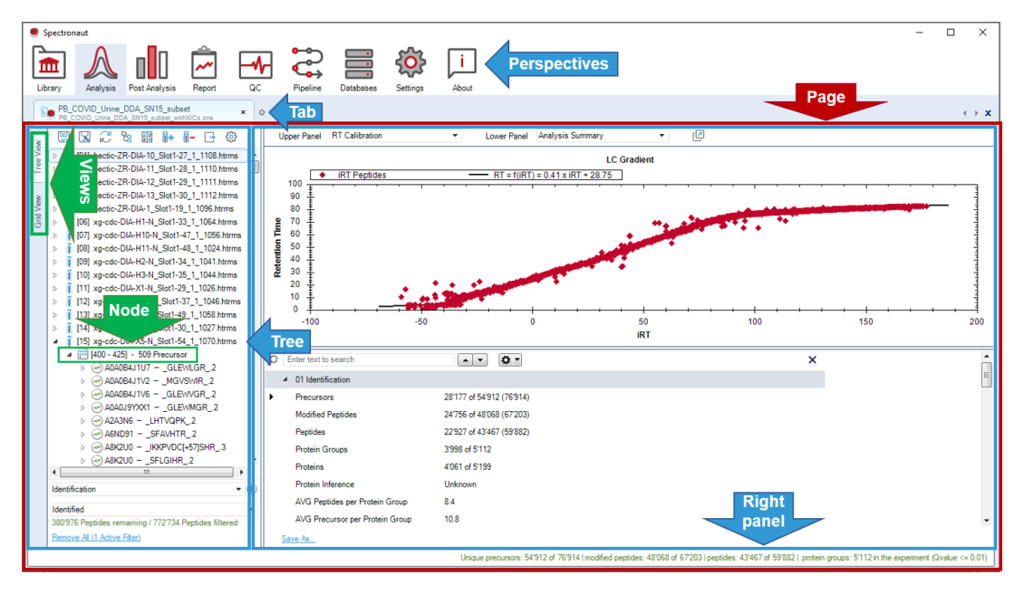
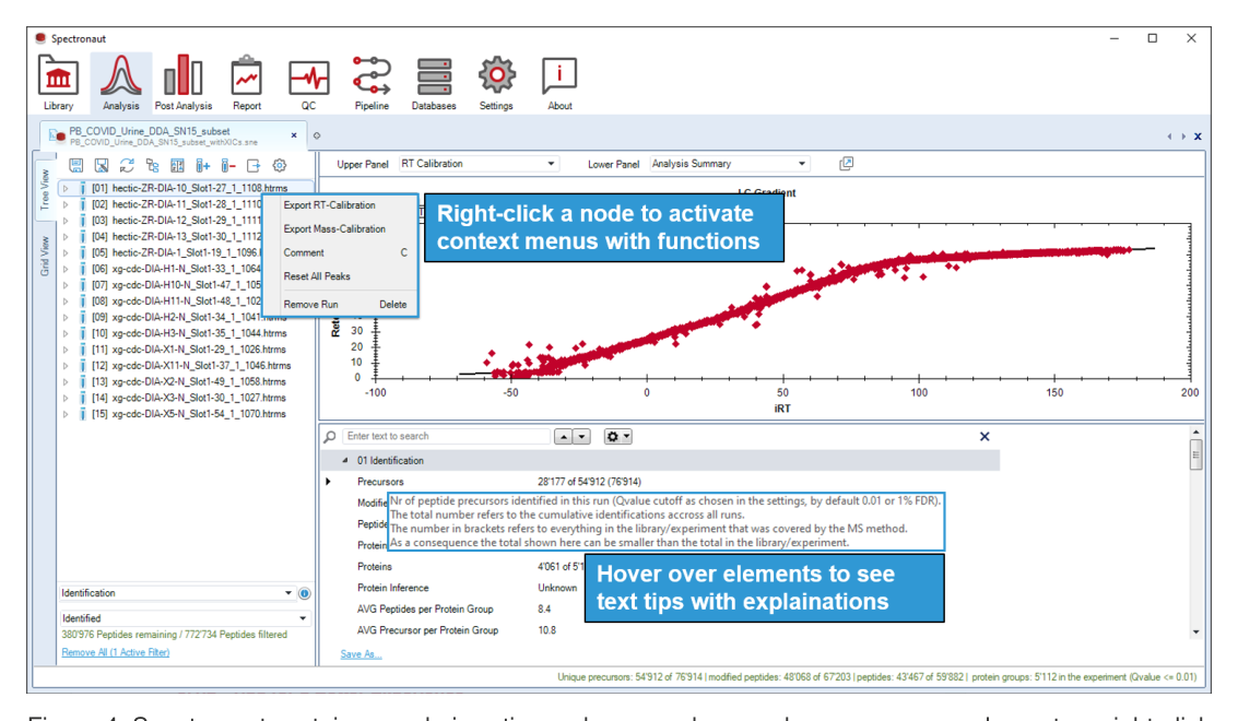
重点:用于界面定位、参数理解或模块功能回查。
重点:用于界面定位、参数理解或模块功能回查。
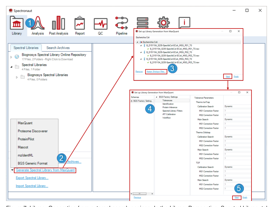
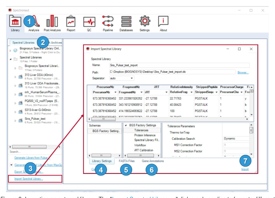
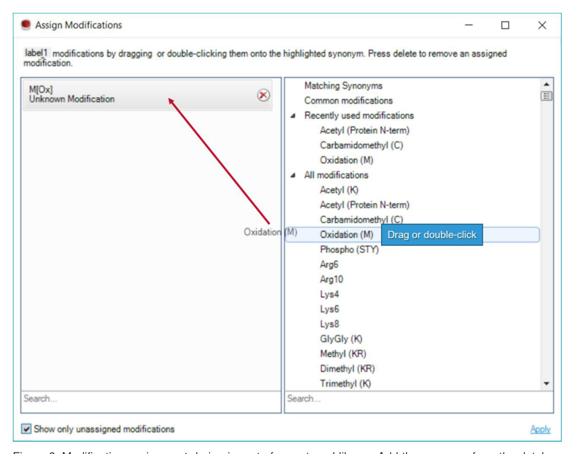
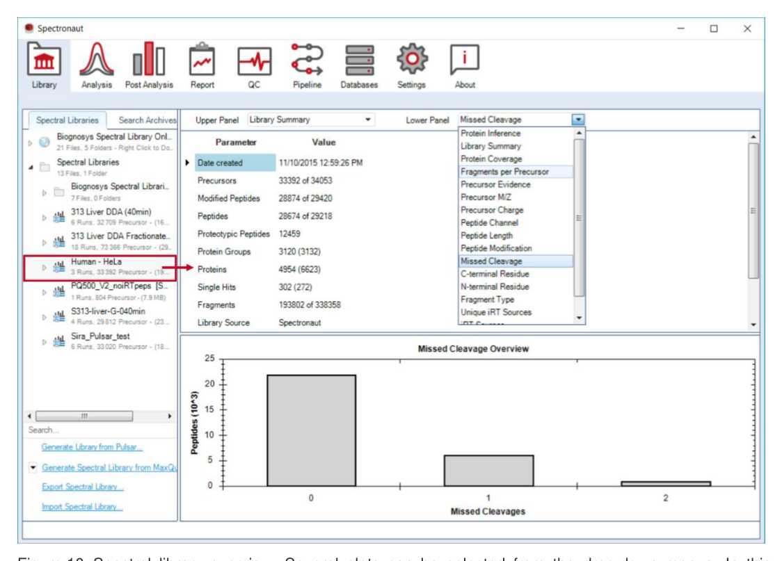
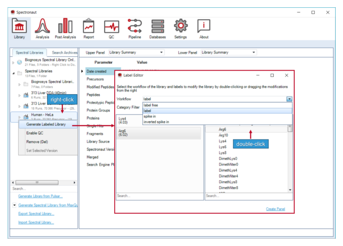
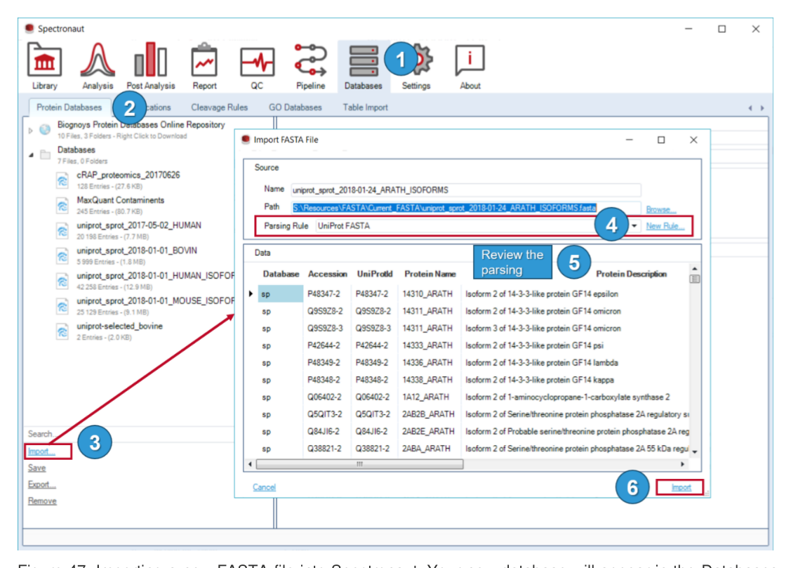
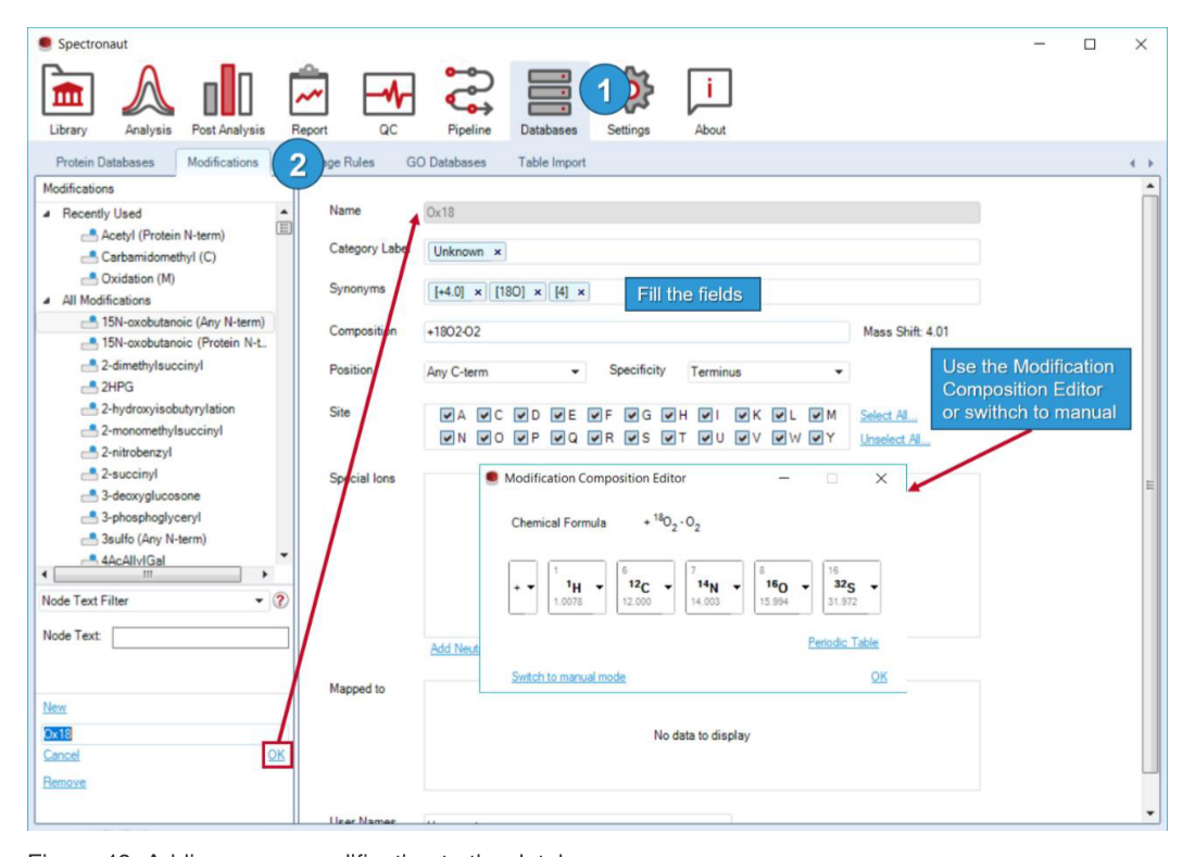
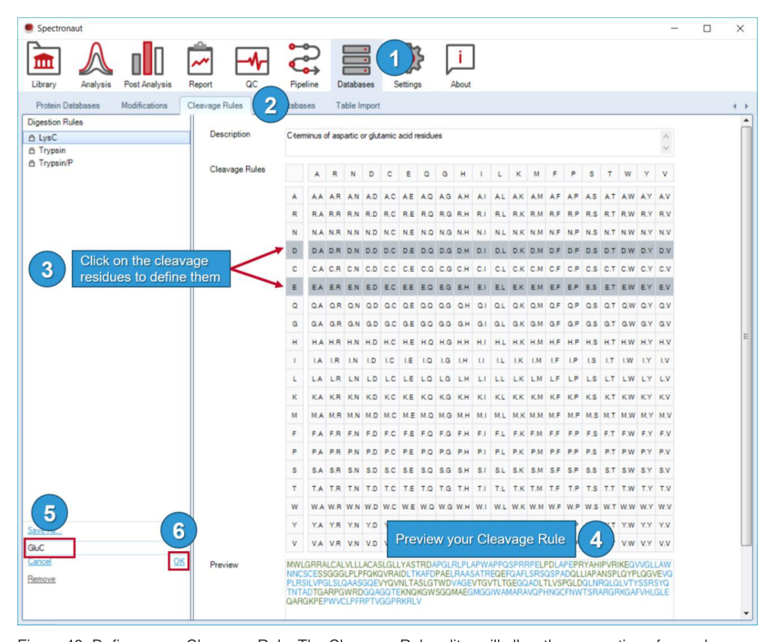
重点:用于谱库构建、外部结果导入和 Search Archive 复用。
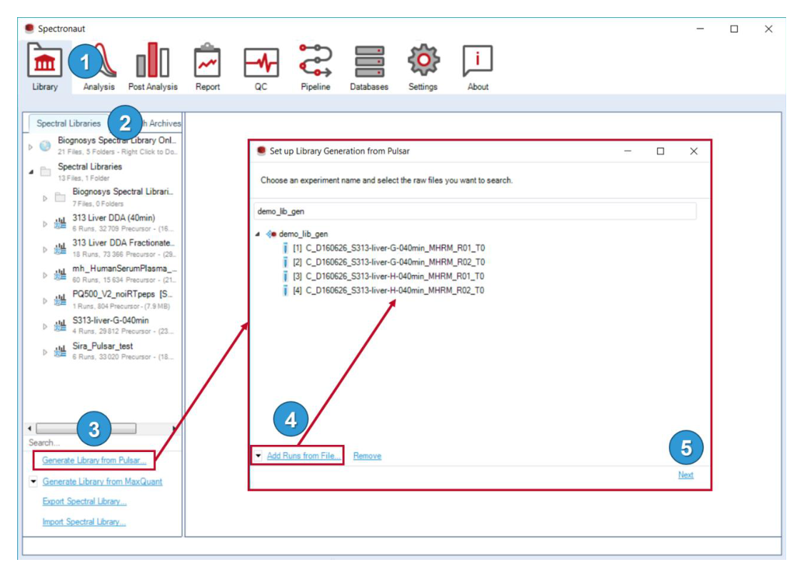
重点:用于谱库构建、外部结果导入和 Search Archive 复用。
图组
Pulsar、外部谱库导入、Search Archive 与 QC kit。
重点:用于谱库构建、外部结果导入和 Search Archive 复用。
重点:用于谱库构建、外部结果导入和 Search Archive 复用。
重点:用于谱库构建、外部结果导入和 Search Archive 复用。
重点:用于谱库构建、外部结果导入和 Search Archive 复用。
重点:用于谱库构建、外部结果导入和 Search Archive 复用。
重点:用于谱库构建、外部结果导入和 Search Archive 复用。
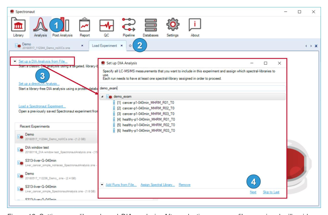
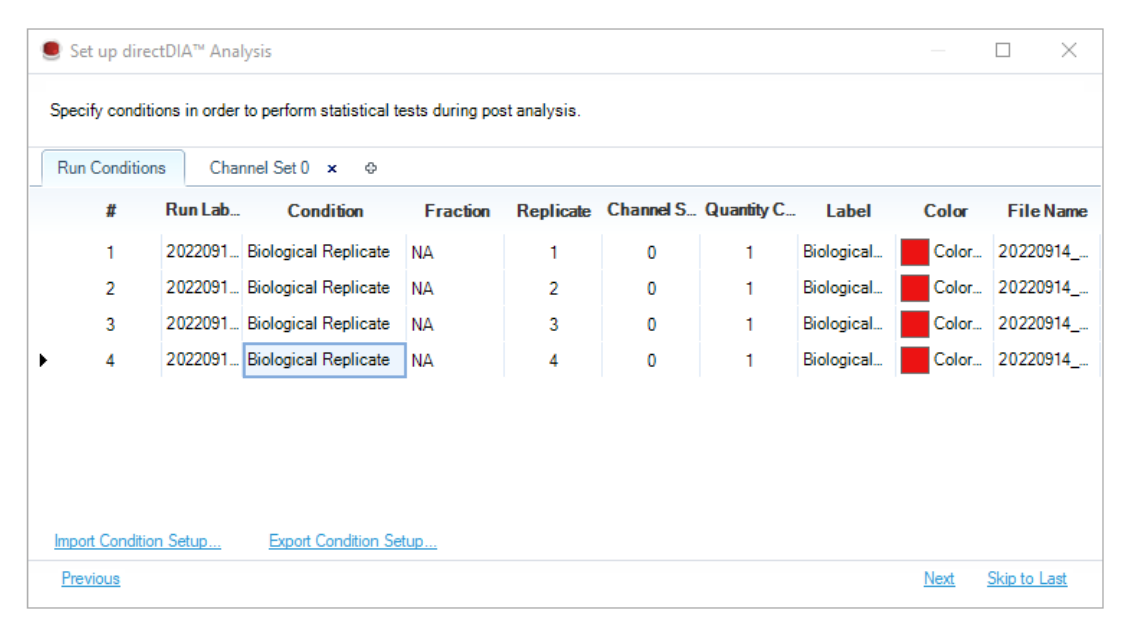
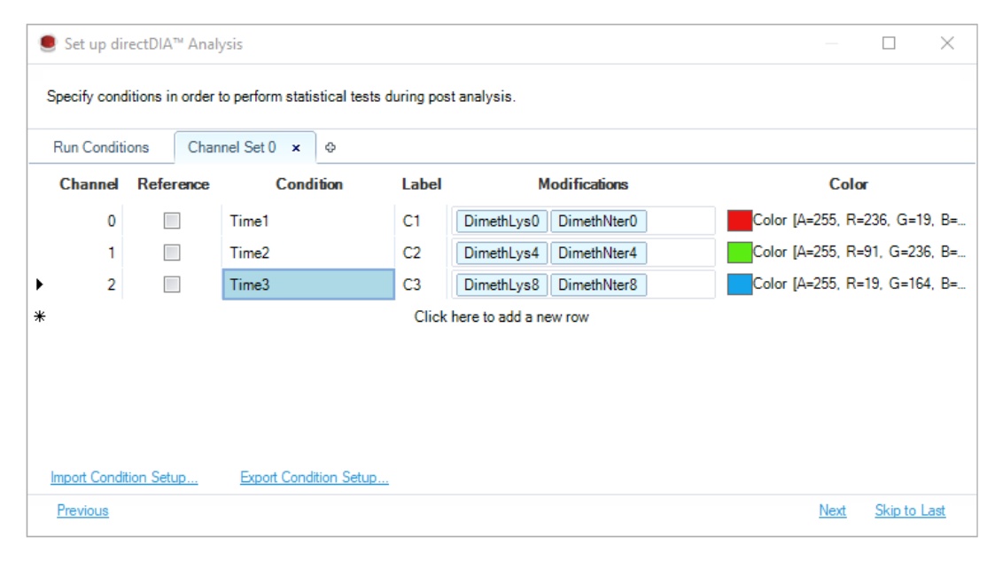
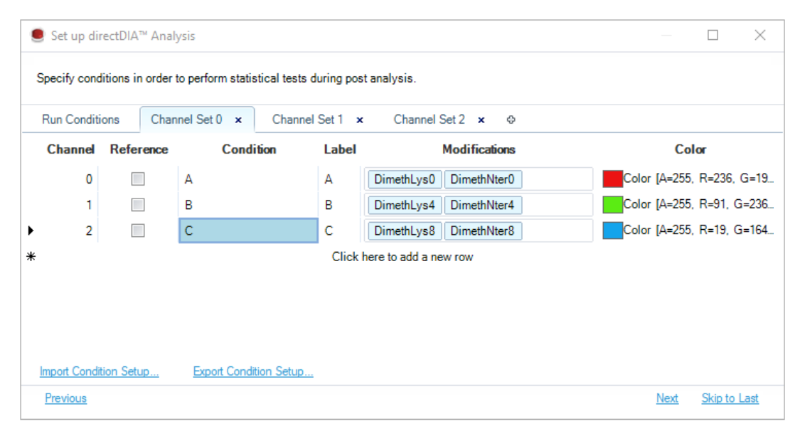
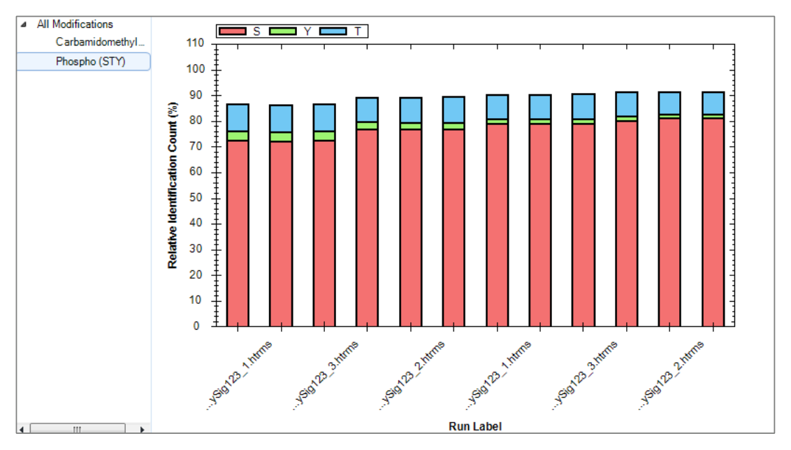
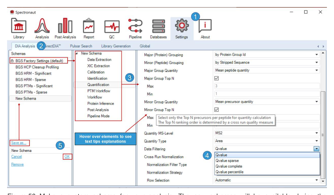
重点:用于选择 workflow、配置条件并执行分析复核。
重点:用于选择 workflow、配置条件并执行分析复核。
重点:用于界面定位、参数理解或模块功能回查。
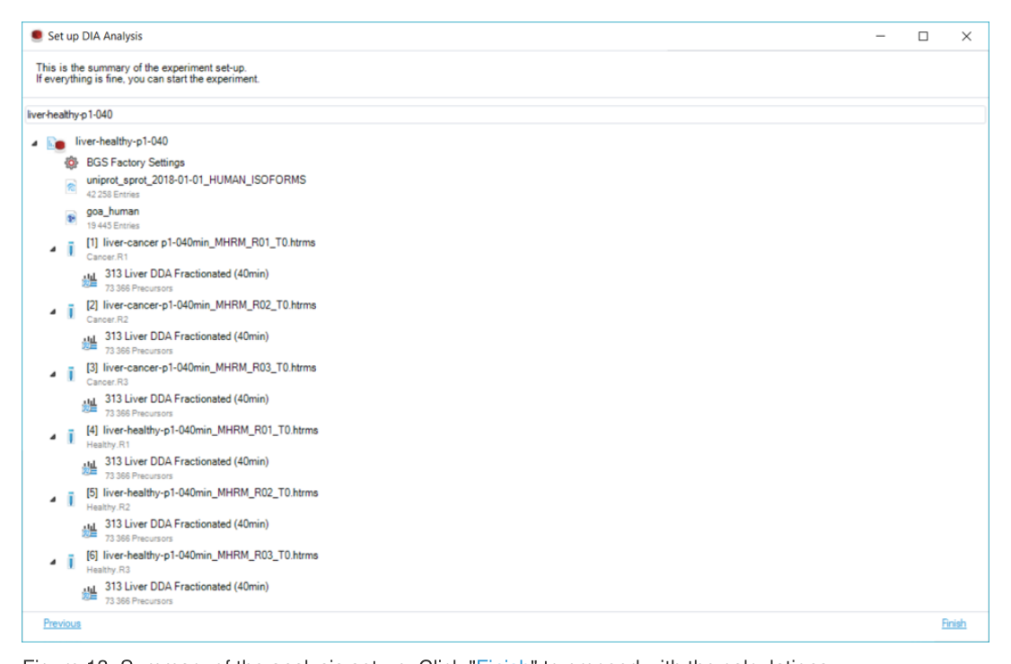
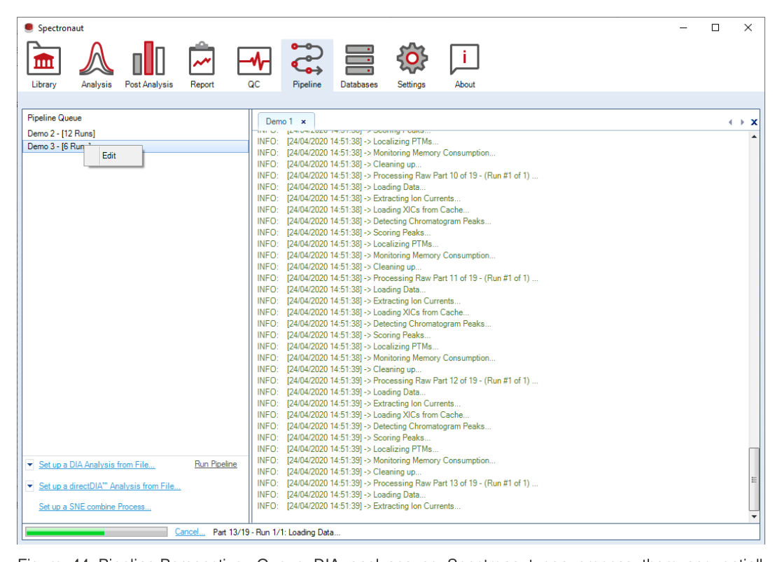
重点:用于选择 workflow、配置条件并执行分析复核。

重点:用于选择 workflow、配置条件并执行分析复核。
图组
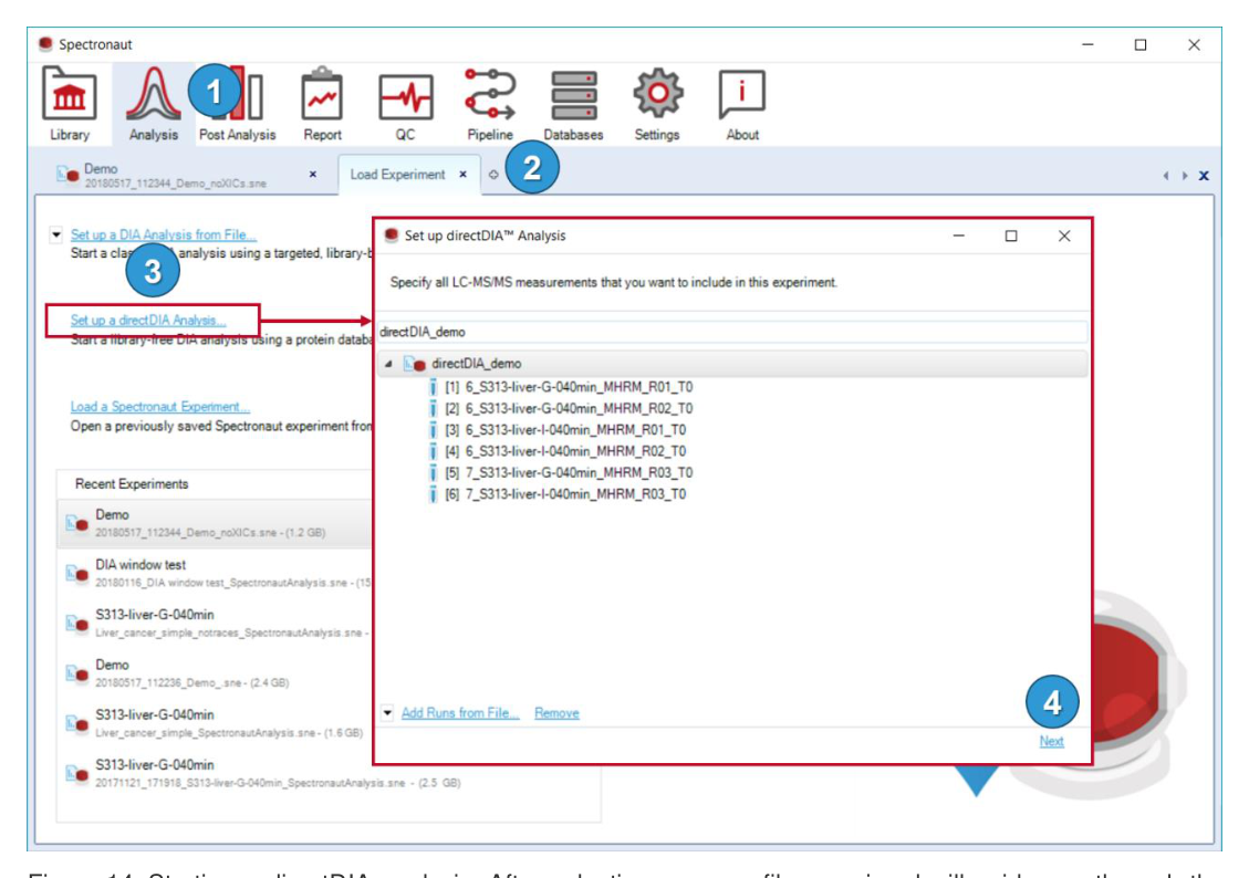
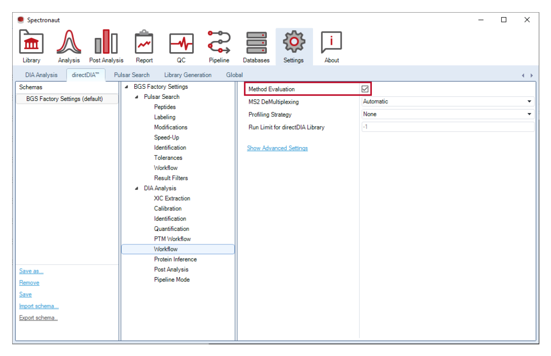
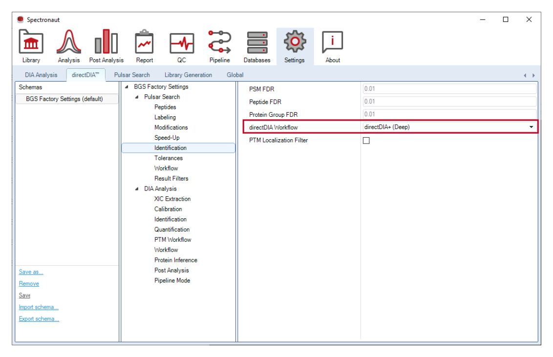
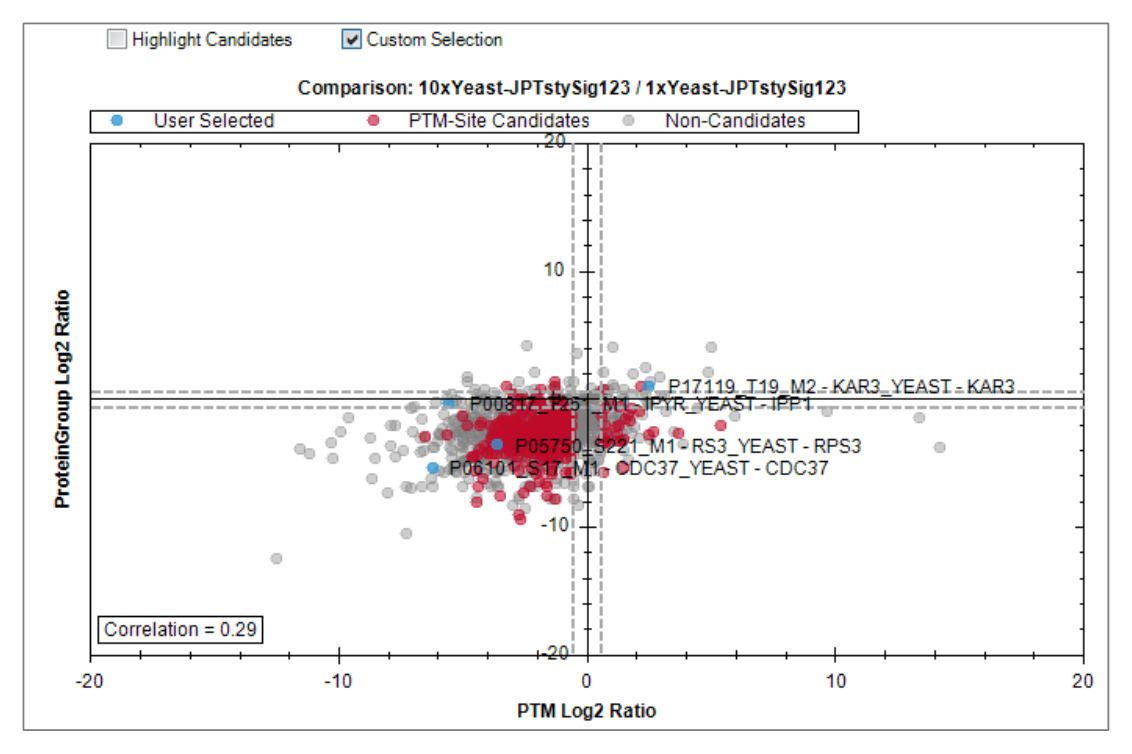
library-based DIA、directDIA、PTM probing 与条件设计。
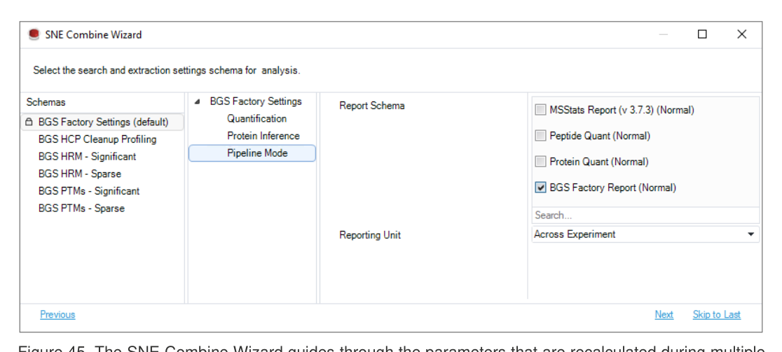
重点:用于选择 workflow、配置条件并执行分析复核。
重点:用于选择 workflow、配置条件并执行分析复核。

重点:用于选择 workflow、配置条件并执行分析复核。
重点:用于选择 workflow、配置条件并执行分析复核。

重点:用于界面定位、参数理解或模块功能回查。
重点:用于选择 workflow、配置条件并执行分析复核。
重点:用于选择 workflow、配置条件并执行分析复核。
重点:用于选择 workflow、配置条件并执行分析复核。
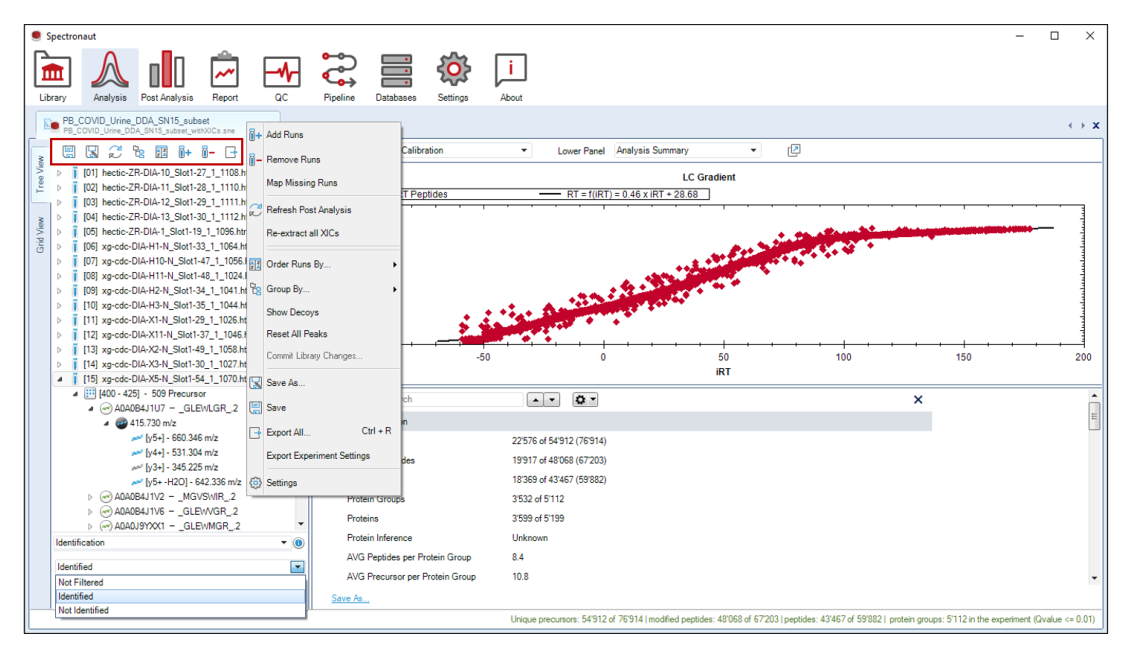
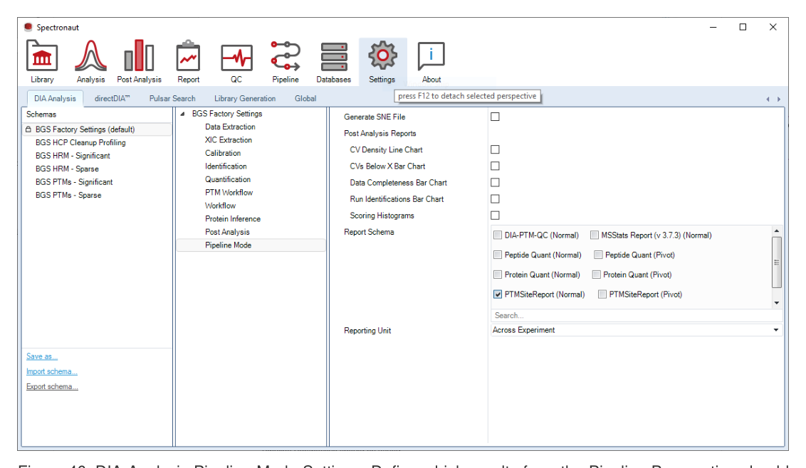
重点:用于界面定位、参数理解或模块功能回查。
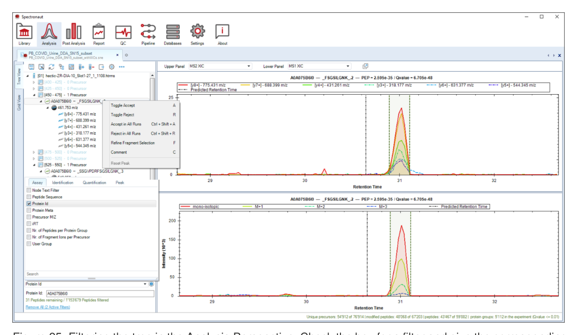
重点:用于界面定位、参数理解或模块功能回查。
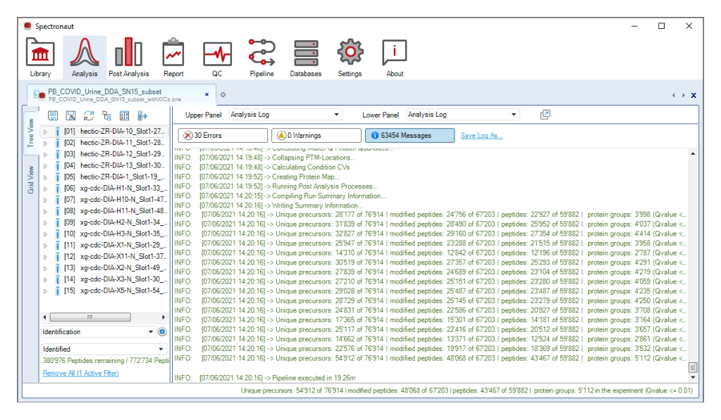
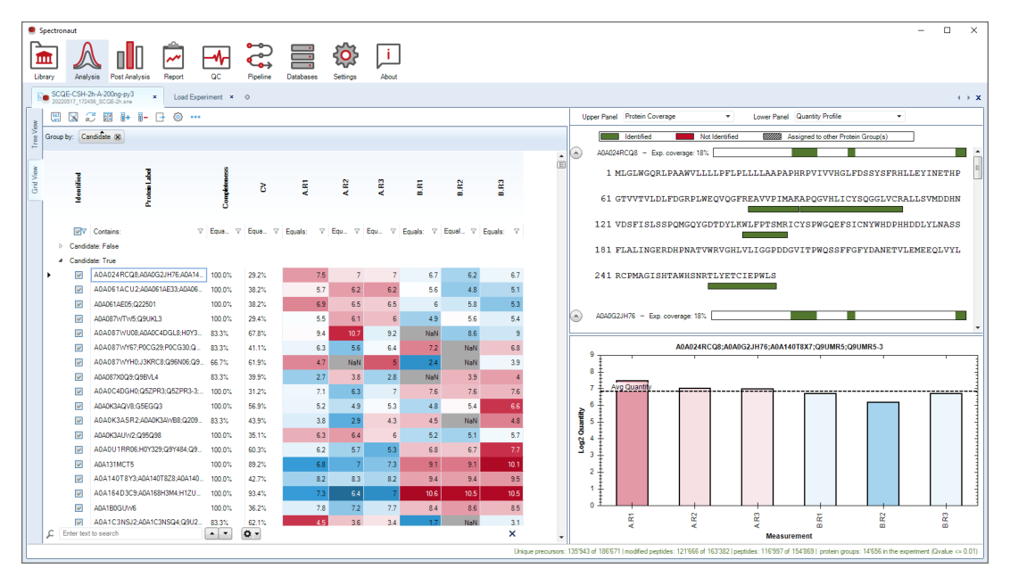
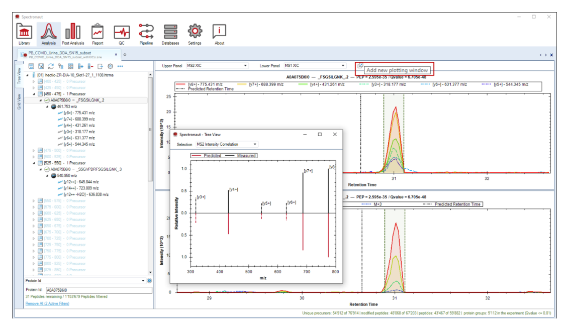
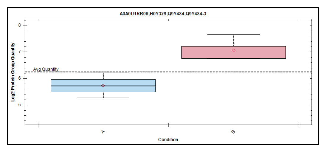
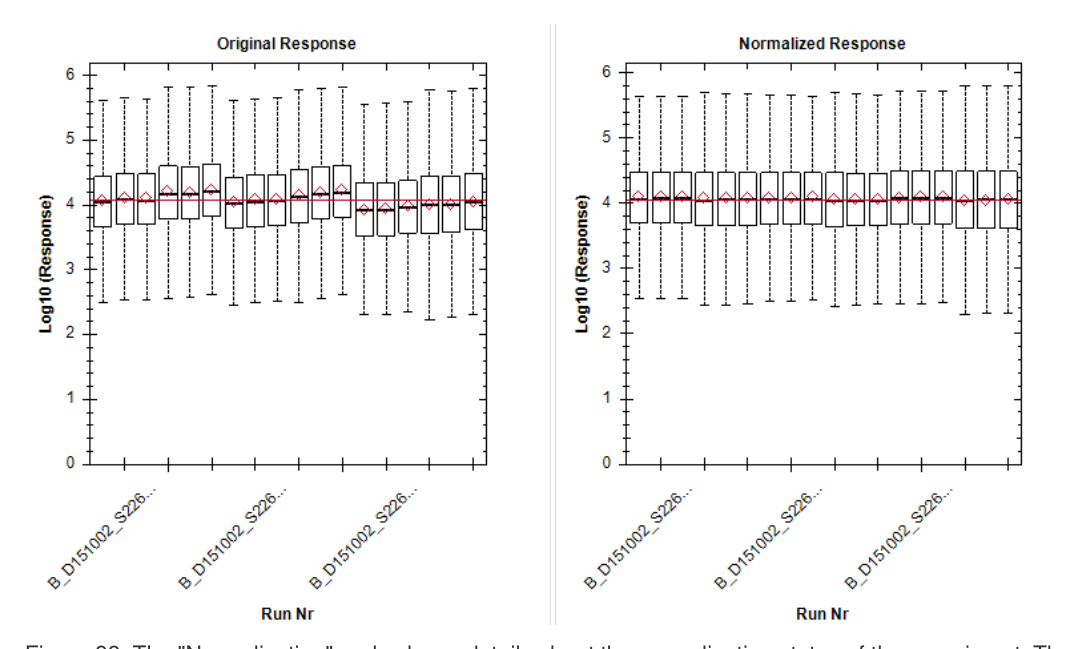
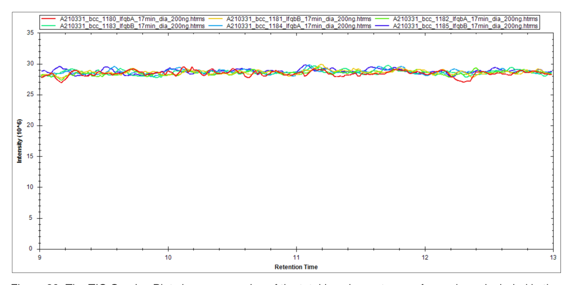
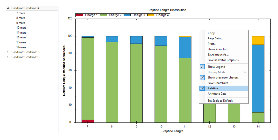
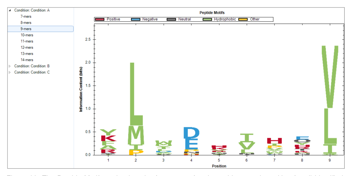
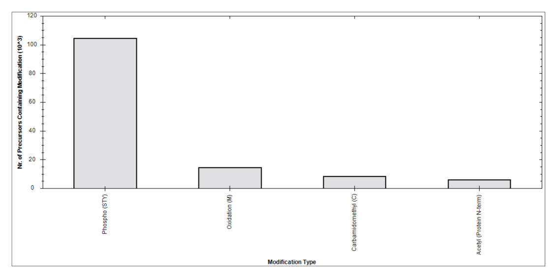
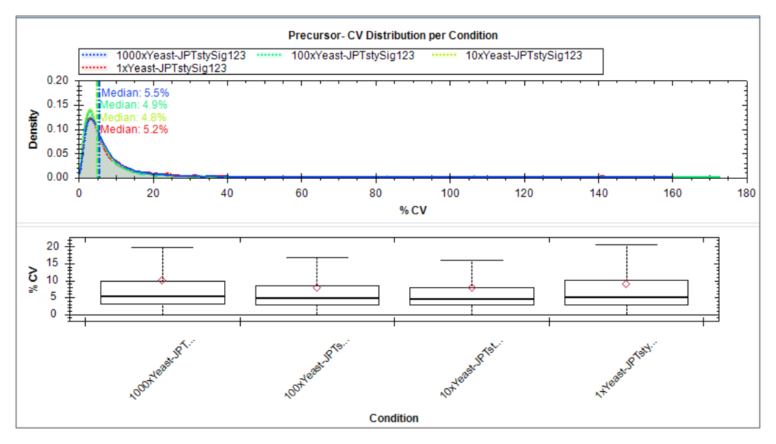
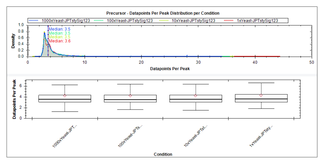
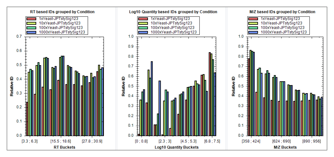
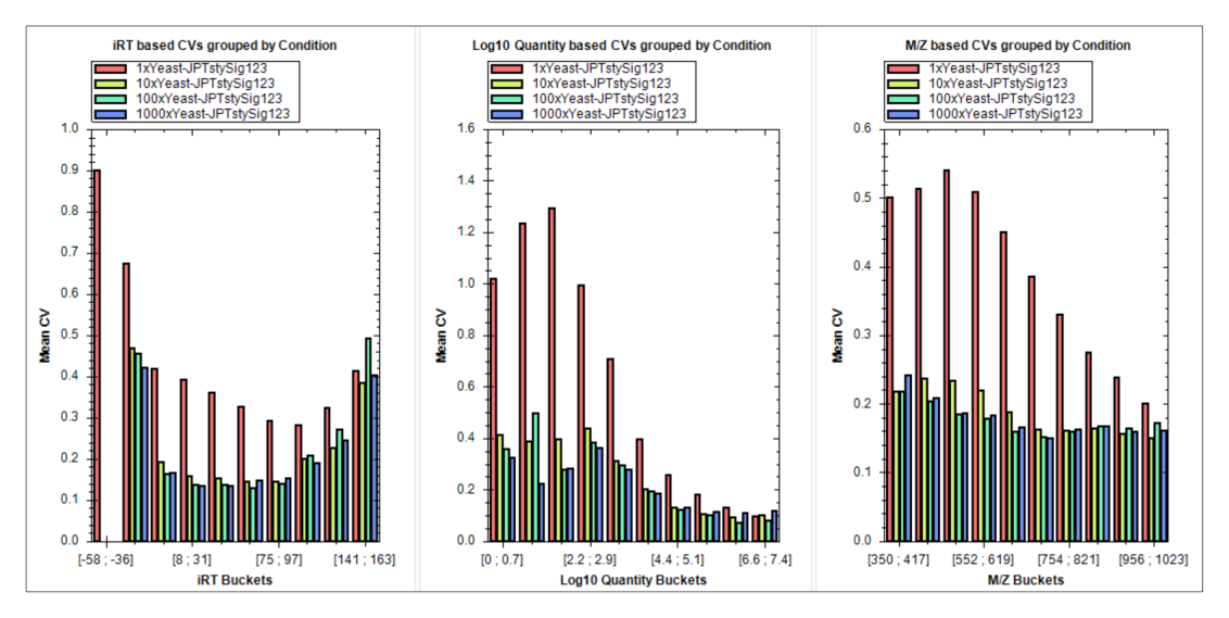
重点:用于结果判读、图谱阅读和差异分析复核。
重点:用于选择 workflow、配置条件并执行分析复核。
重点:用于选择 workflow、配置条件并执行分析复核。
重点:用于界面定位、参数理解或模块功能回查。
重点:用于谱库构建、外部结果导入和 Search Archive 复用。
重点:用于选择 workflow、配置条件并执行分析复核。
重点:用于选择 workflow、配置条件并执行分析复核。
图组
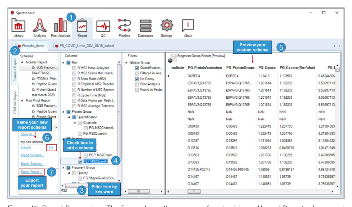
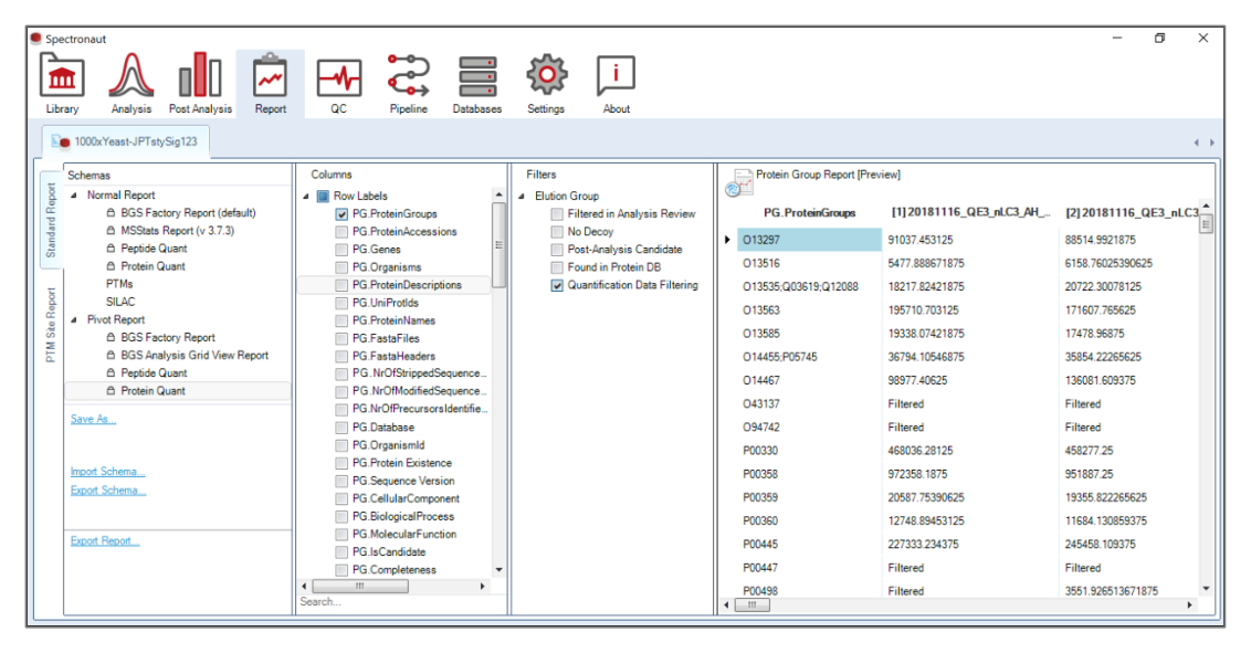
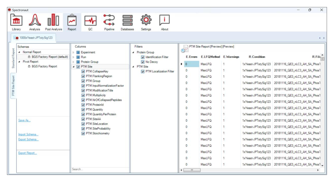
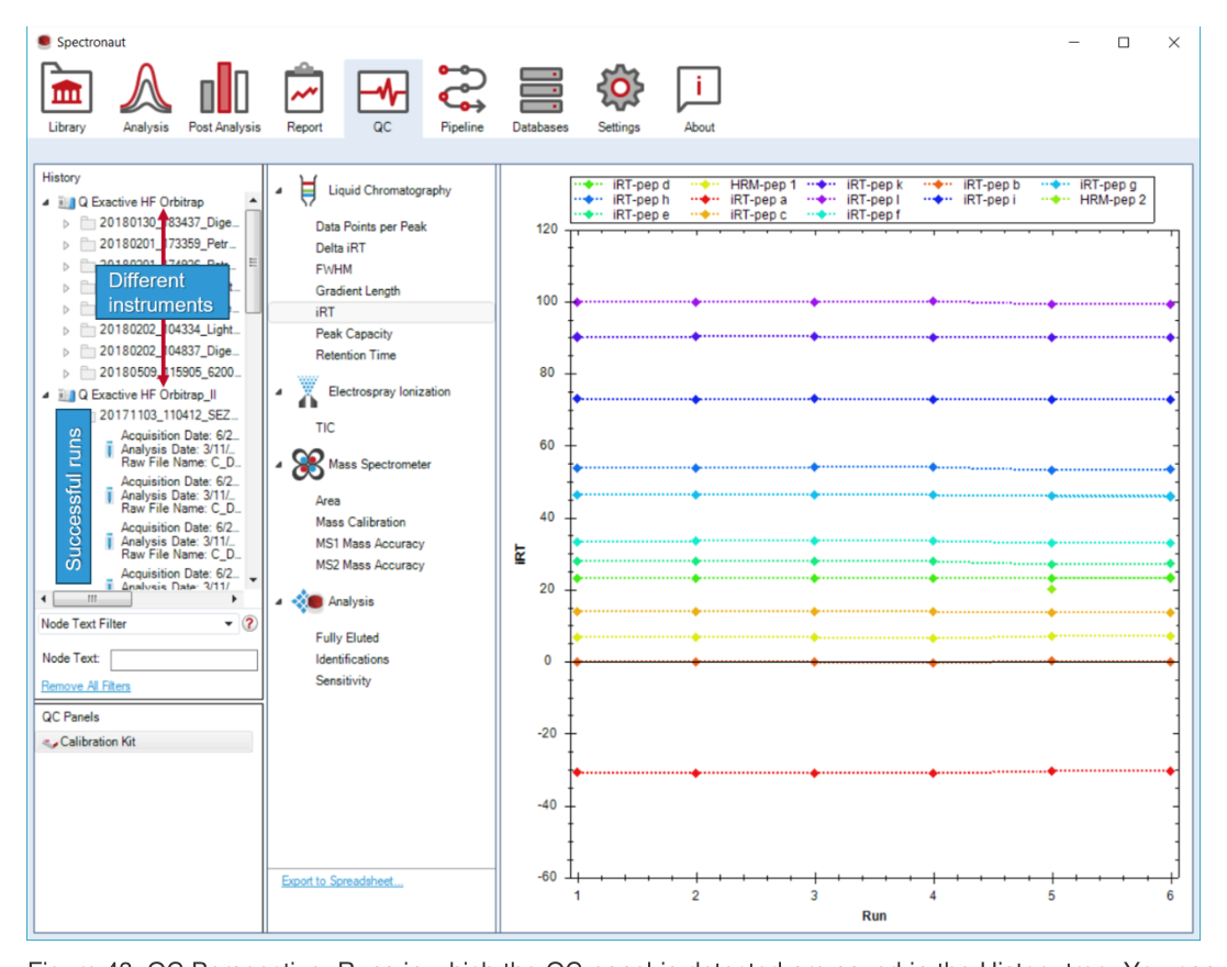
报表结构、QC 模块、数据库与修饰规则管理。
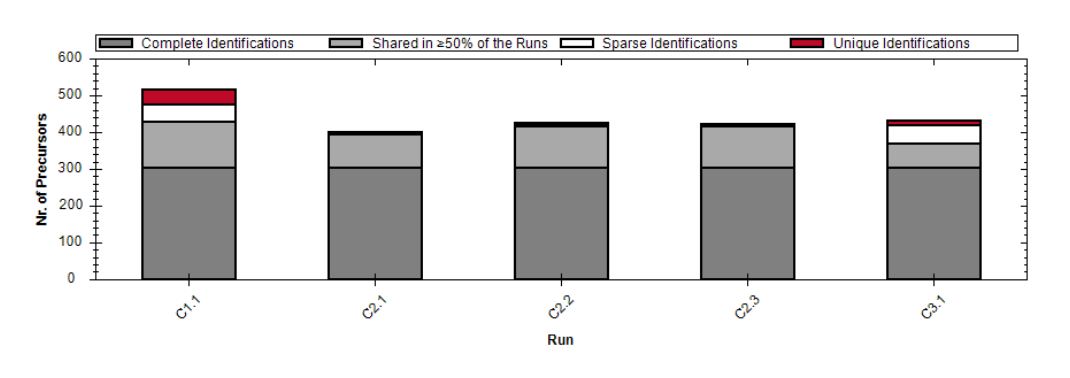
重点:用于结果判读、图谱阅读和差异分析复核。
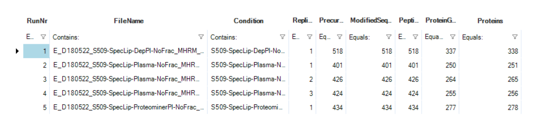
重点:用于结果判读、图谱阅读和差异分析复核。
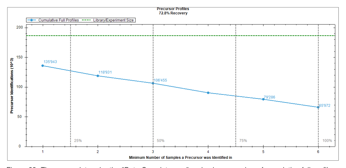
重点:用于结果判读、图谱阅读和差异分析复核。
重点:用于报表导出、QC 监控、数据库与字段管理。
重点:用于选择 workflow、配置条件并执行分析复核。
重点:用于报表导出、QC 监控、数据库与字段管理。
重点:用于报表导出、QC 监控、数据库与字段管理。
重点:用于选择 workflow、配置条件并执行分析复核。
重点:用于报表导出、QC 监控、数据库与字段管理。
重点:用于界面定位、参数理解或模块功能回查。
重点:用于界面定位、参数理解或模块功能回查。
重点:用于选择 workflow、配置条件并执行分析复核。
重点:用于报表导出、QC 监控、数据库与字段管理。
重点:用于报表导出、QC 监控、数据库与字段管理。
重点:用于报表导出、QC 监控、数据库与字段管理。
重点:用于选择 workflow、配置条件并执行分析复核。
重点:用于界面定位、参数理解或模块功能回查。
重点:用于界面定位、参数理解或模块功能回查。
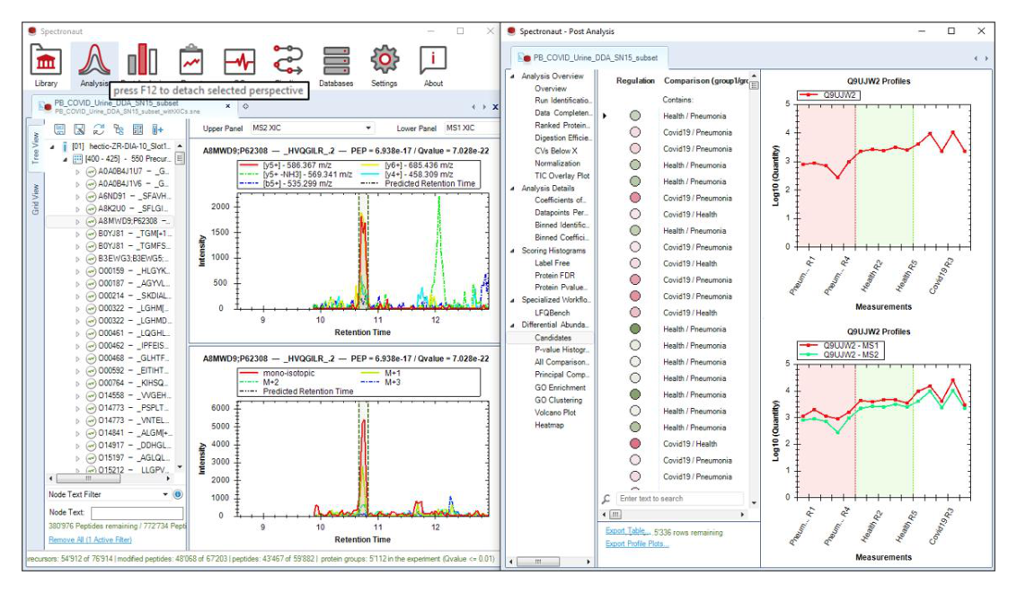
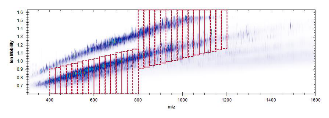
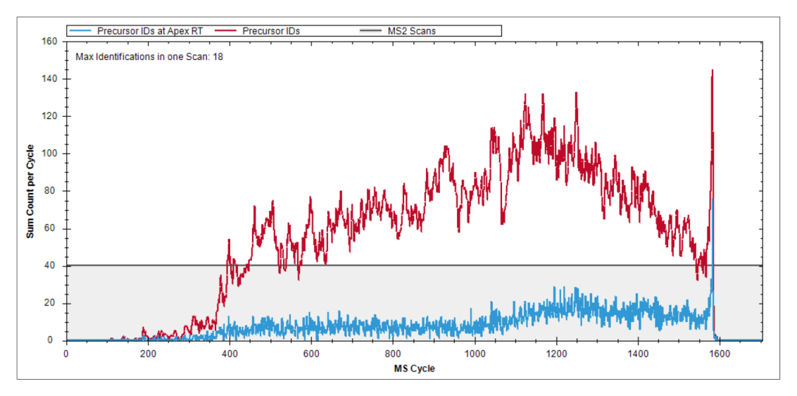
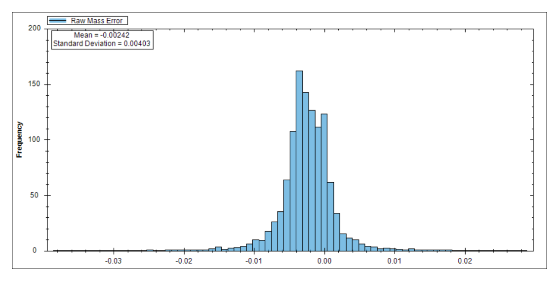
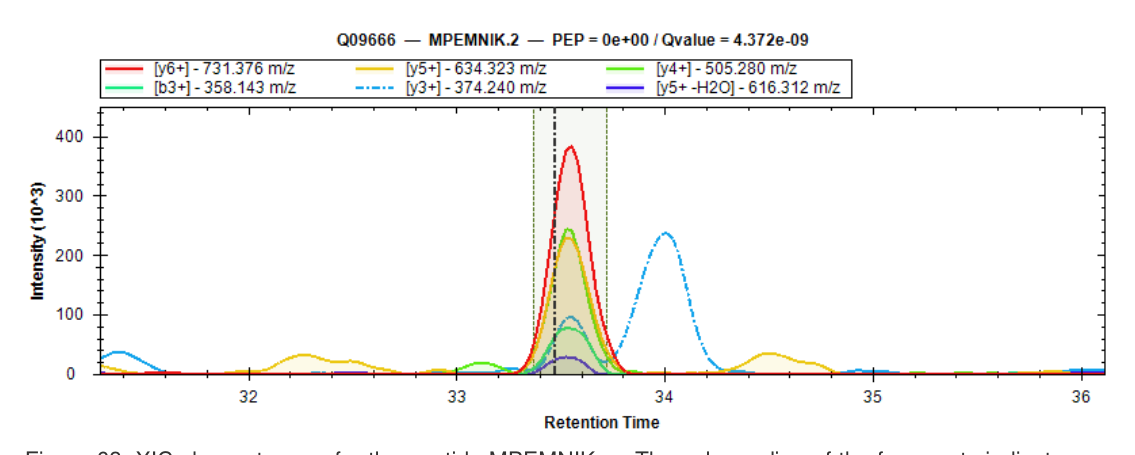
图组
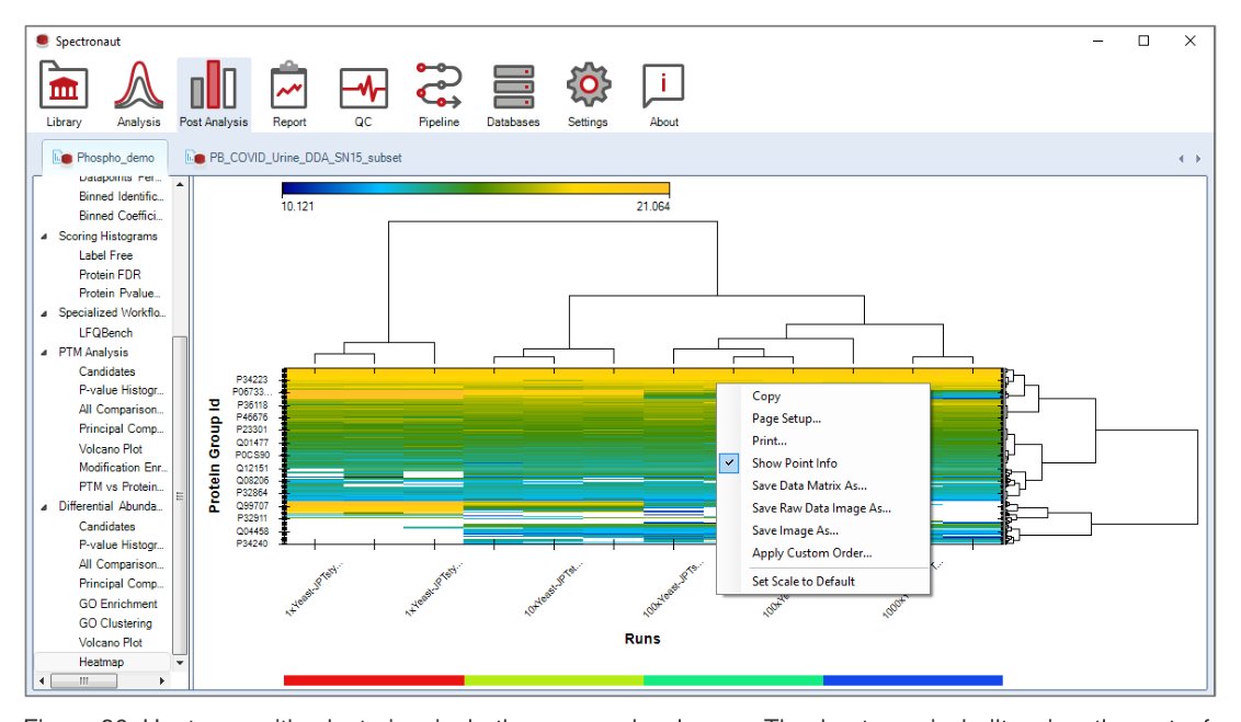
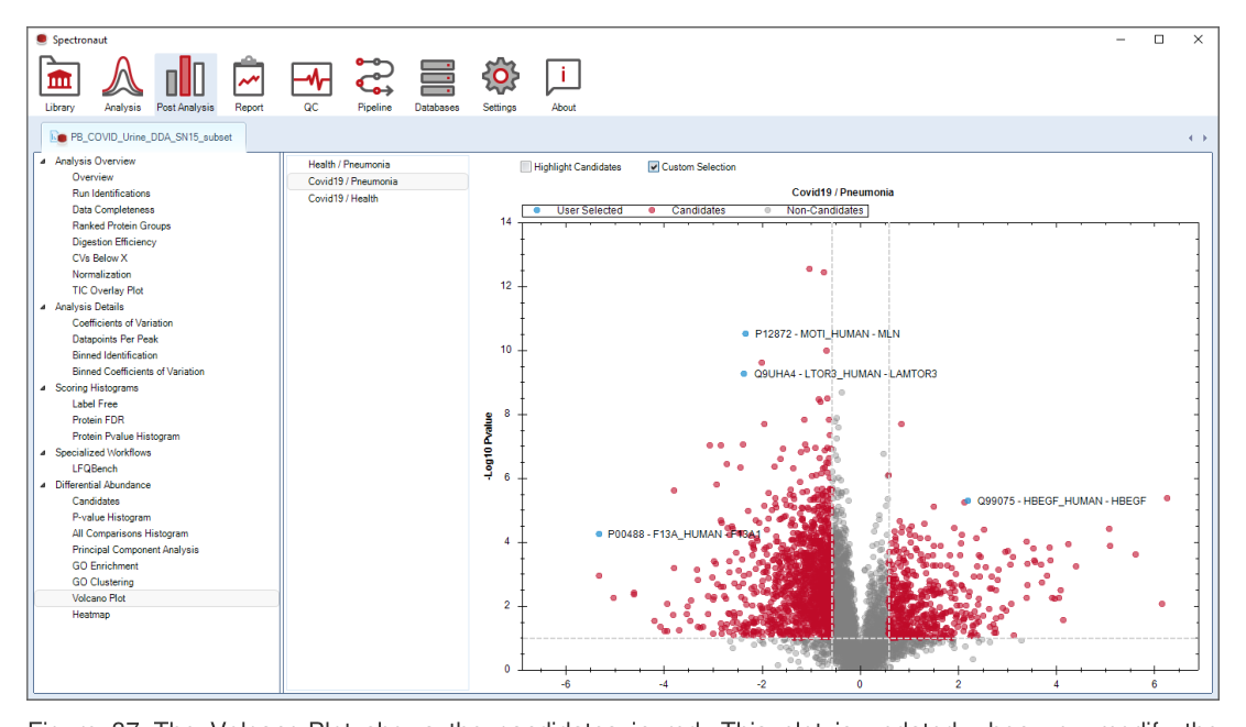
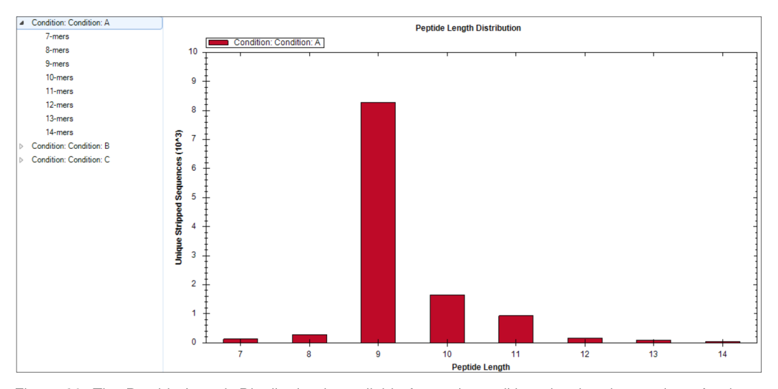
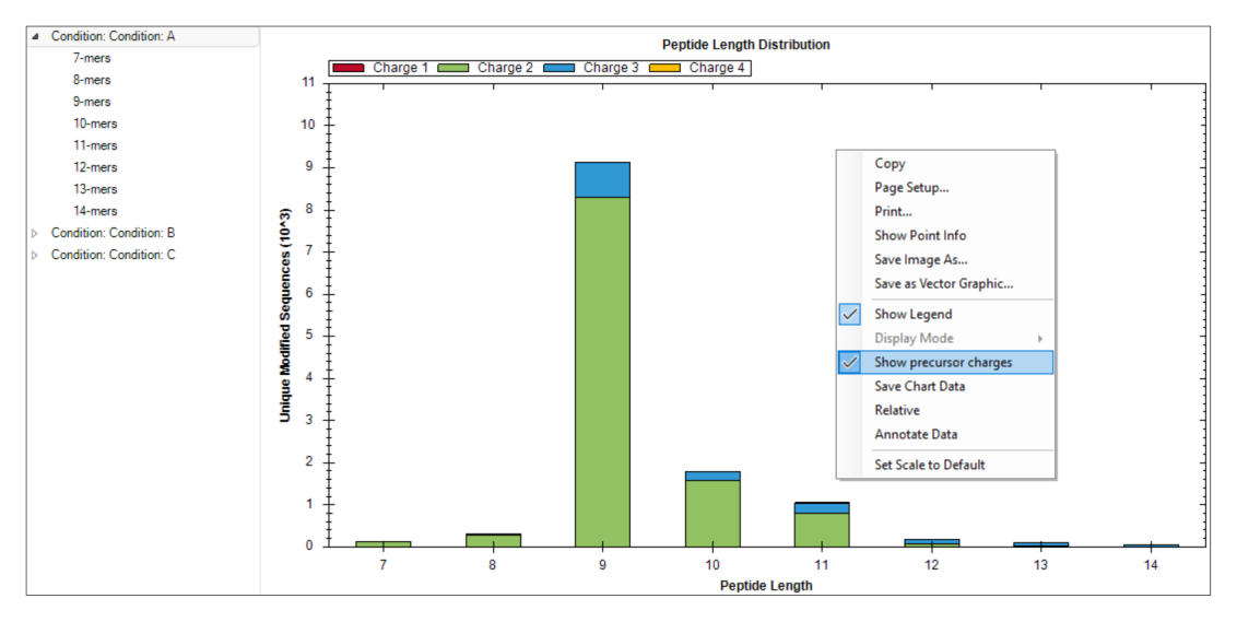
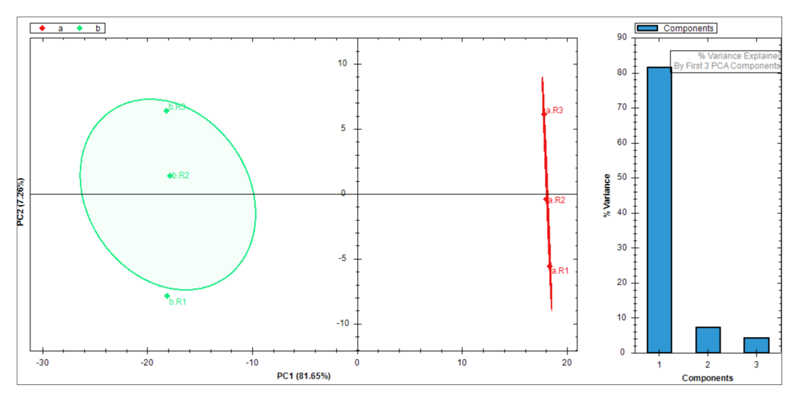
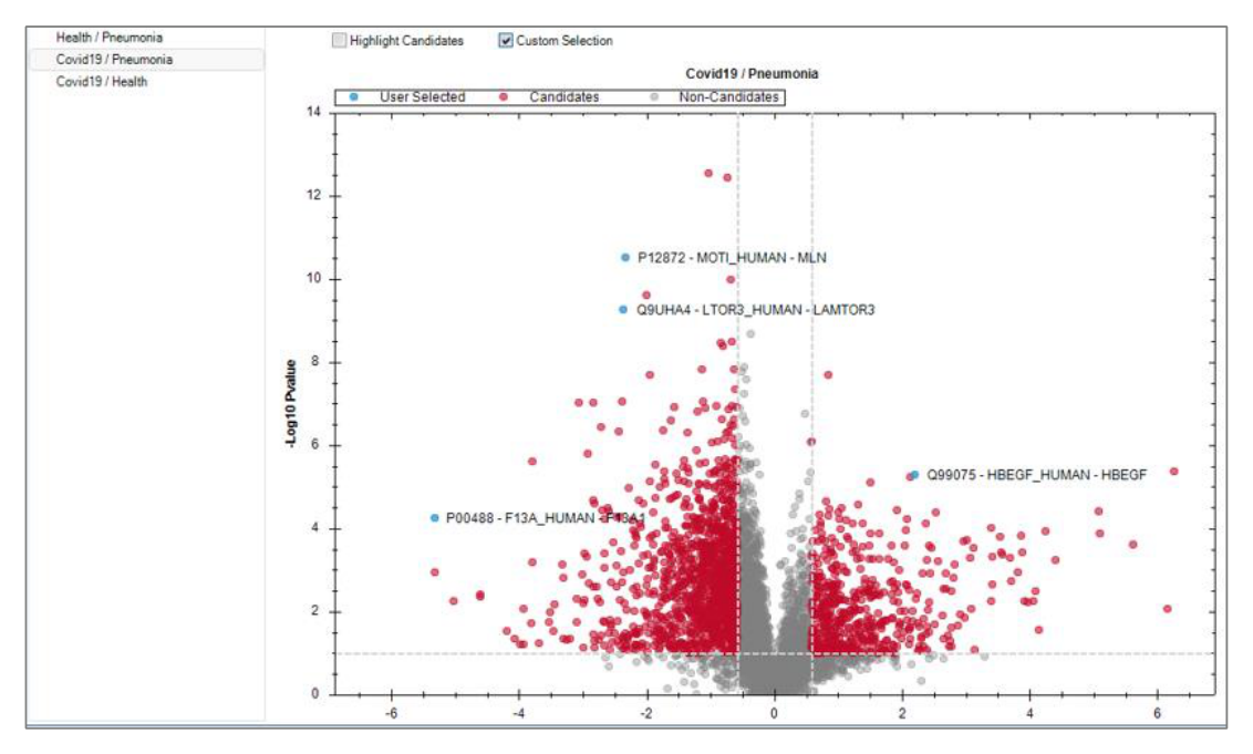
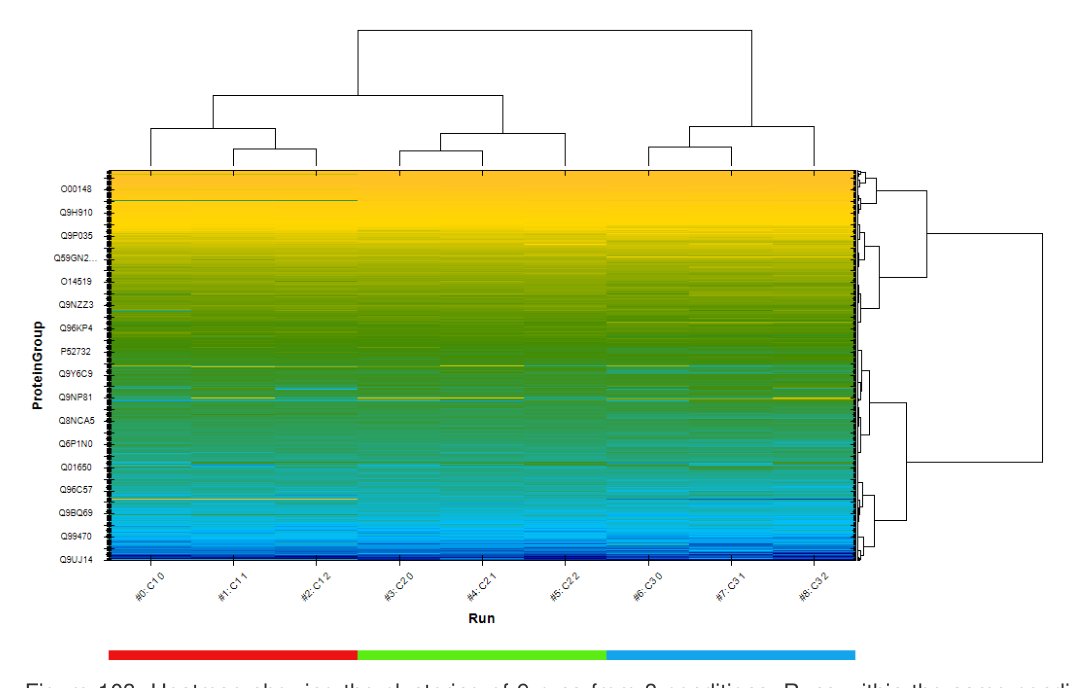
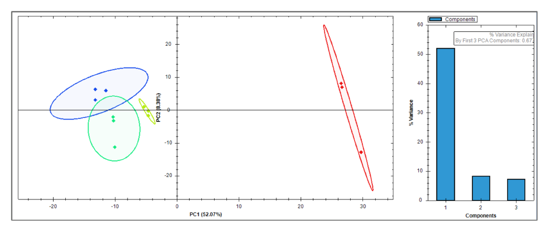
Candidates、PCA、heatmap、volcano、coverage 与 XIC。
重点:用于谱库构建、外部结果导入和 Search Archive 复用。
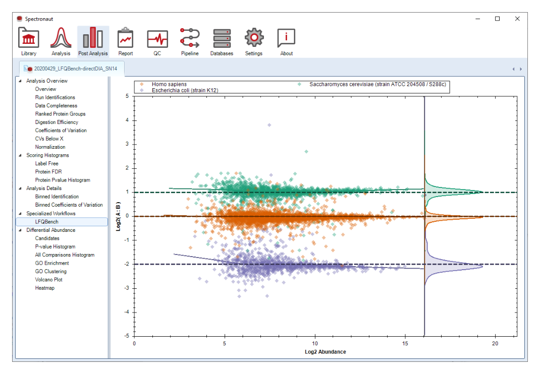
重点:用于结果判读、图谱阅读和差异分析复核。
重点:用于界面定位、参数理解或模块功能回查。
重点:用于界面定位、参数理解或模块功能回查。
重点:用于界面定位、参数理解或模块功能回查。
重点:用于选择 workflow、配置条件并执行分析复核。
重点:用于界面定位、参数理解或模块功能回查。
重点:用于界面定位、参数理解或模块功能回查。
重点:用于界面定位、参数理解或模块功能回查。
重点:用于界面定位、参数理解或模块功能回查。
重点:用于结果判读、图谱阅读和差异分析复核。
重点:用于结果判读、图谱阅读和差异分析复核。
重点:用于界面定位、参数理解或模块功能回查。
重点:用于界面定位、参数理解或模块功能回查。
重点:用于结果判读、图谱阅读和差异分析复核。
重点:用于界面定位、参数理解或模块功能回查。
重点:用于选择 workflow、配置条件并执行分析复核。
重点:用于界面定位、参数理解或模块功能回查。
重点:用于界面定位、参数理解或模块功能回查。
重点:用于界面定位、参数理解或模块功能回查。
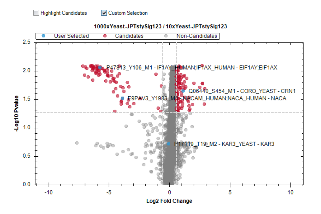
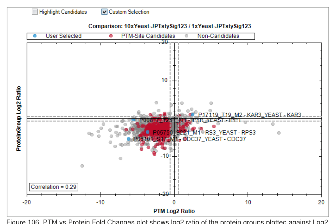
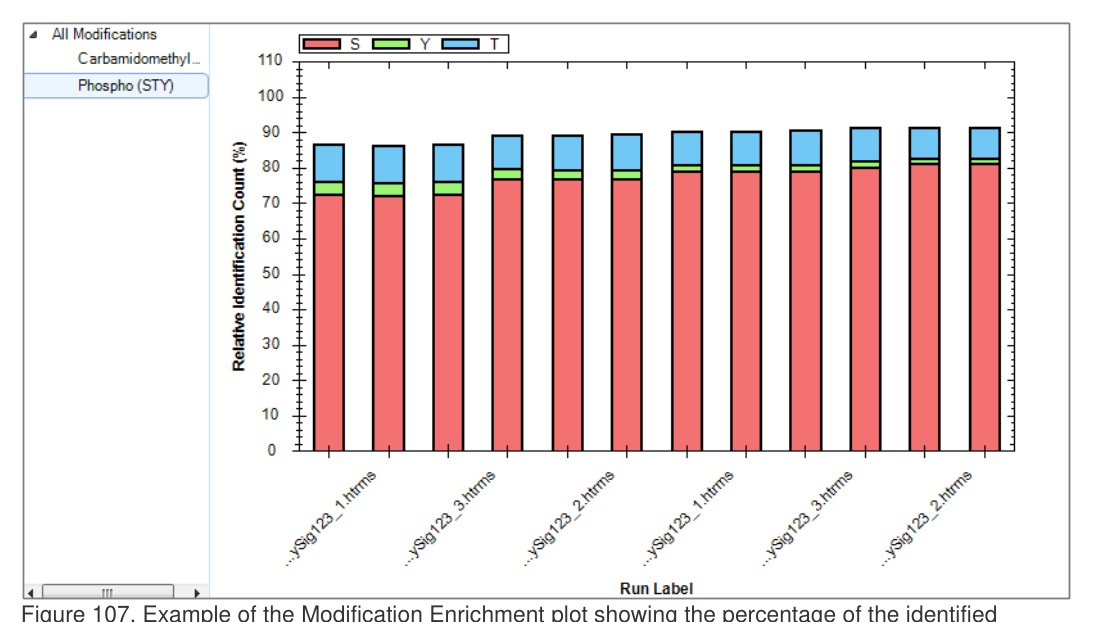
重点:用于结果判读、图谱阅读和差异分析复核。
重点:用于结果判读、图谱阅读和差异分析复核。
重点:用于结果判读、图谱阅读和差异分析复核。
重点:用于界面定位、参数理解或模块功能回查。
重点:用于界面定位、参数理解或模块功能回查。
重点:用于界面定位、参数理解或模块功能回查。
重点:用于结果判读、图谱阅读和差异分析复核。
重点:用于选择 workflow、配置条件并执行分析复核。
图组
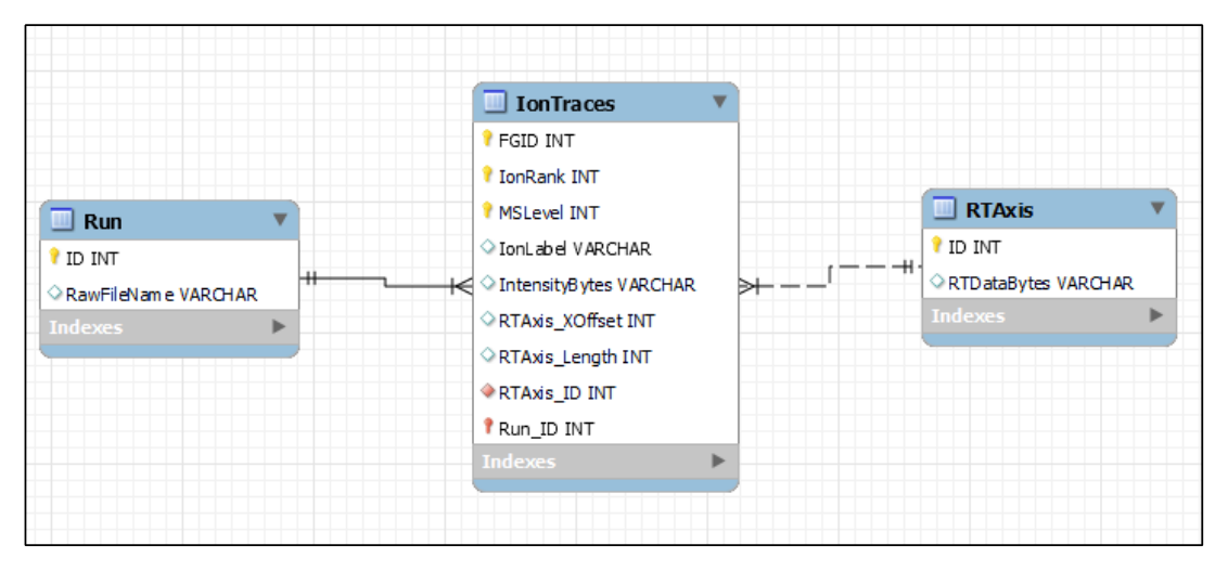
Appendix 图谱、字段解释、XIC 数据库与导出结构。
重点:用于界面定位、参数理解或模块功能回查。
重点:用于界面定位、参数理解或模块功能回查。
重点:用于结果判读、图谱阅读和差异分析复核。
重点:用于结果判读、图谱阅读和差异分析复核。
重点:用于界面定位、参数理解或模块功能回查。
重点:用于界面定位、参数理解或模块功能回查。
重点:用于界面定位、参数理解或模块功能回查。
重点:用于界面定位、参数理解或模块功能回查。
重点:用于界面定位、参数理解或模块功能回查。
重点:用于选择 workflow、配置条件并执行分析复核。
重点:用于界面定位、参数理解或模块功能回查。
重点:用于界面定位、参数理解或模块功能回查。
重点:用于界面定位、参数理解或模块功能回查。
重点:用于报表导出、QC 监控、数据库与字段管理。
重点:用于界面定位、参数理解或模块功能回查。
重点:用于选择 workflow、配置条件并执行分析复核。
重点:用于界面定位、参数理解或模块功能回查。
重点:用于界面定位、参数理解或模块功能回查。
重点:用于界面定位、参数理解或模块功能回查。

重点:用于界面定位、参数理解或模块功能回查。
重点:用于选择 workflow、配置条件并执行分析复核。
重点:用于选择 workflow、配置条件并执行分析复核。
重点:用于选择 workflow、配置条件并执行分析复核。
重点:用于选择 workflow、配置条件并执行分析复核。
重点:用于选择 workflow、配置条件并执行分析复核。
重点:用于选择 workflow、配置条件并执行分析复核。
重点:用于报表导出、QC 监控、数据库与字段管理。
重点:用于报表导出、QC 监控、数据库与字段管理。